Compute a radio map

Build a two-room indoor scene, compute a coverage map with the deterministic and Monte Carlo solvers, and plot it in dB.

This guide computes the coverage of one access point in two rooms joined by a door. It shows how to build walls, define a grid, run two solvers and plot the result. Read Radio maps first for the grid layout.

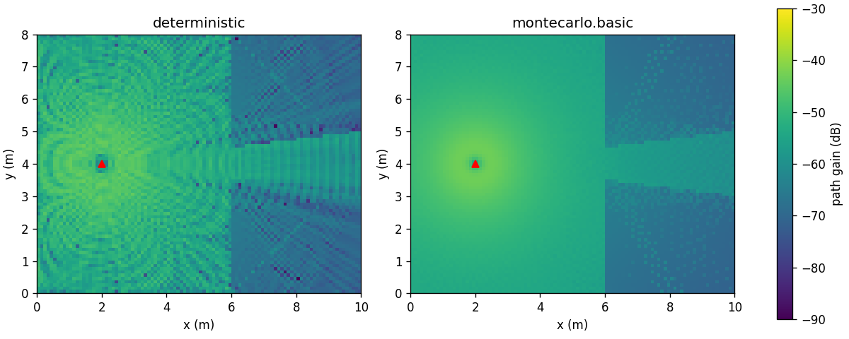Deterministic and Monte Carlo radio maps of two rooms

The script #

You need matplotlib for the plot (pip install matplotlib).

import torch
import matplotlib.pyplot as plt
 
from witwin.core import AntennaState, Mesh, PhysicalMaterial, ReceiverGrid, Scene, Structure
from witwin.channel import deterministic
from witwin.channel.montecarlo import basic
 
FREQUENCY_HZ = 3.5e9
concrete = PhysicalMaterial(eps_r=5.24, sigma_e=0.0462, thickness_m=0.2, name="concrete")
 
 
def wall(x0, y0, x1, y1, material, height=3.0):
    """A vertical wall from (x0, y0) to (x1, y1), from z = 0 to z = height."""
    vertices = torch.tensor([
        [x0, y0, 0.0], [x1, y1, 0.0], [x0, y0, height], [x1, y1, height],
    ])
    faces = torch.tensor([[0, 1, 2], [1, 3, 2]])
    return Structure(Mesh(vertices, faces, recenter=False, fill_mode="surface"), material)
 
 
structures = [
    wall(0, 0, 10, 0, concrete), wall(10, 0, 10, 8, concrete),
    wall(10, 8, 0, 8, concrete), wall(0, 8, 0, 0, concrete),
    wall(6, 0, 6, 3.5, concrete), wall(6, 4.5, 6, 8, concrete),  # inner wall with a 1 m door
]
tx = AntennaState(1, "tx", torch.tensor([2.0, 4.0, 2.0]), power_w=1.0)
 
# 100 x 80 samples at 0.1 m spacing, 1.5 m above the floor.
rows, columns = 100, 80
grid = ReceiverGrid(
    2,
    torch.tensor([0.05, 0.05, 1.5]),
    torch.tensor([1.0, 0.0, 0.0]),   # rows step along +x
    torch.tensor([0.0, 1.0, 0.0]),   # columns step along +y
    (rows, columns),
    (0.1, 0.1),
)
scene = Scene(structures=structures, endpoints=[tx, grid])
components = {"los", "reflection", "diffraction", "transmission"}
 
det = deterministic.solve(
    scene,
    deterministic.Config(max_depth=2, components=components),
    reference_frequency_hz=FREQUENCY_HZ,
)
mc = basic.solve(
    scene,
    basic.Config(samples=1_000_000, max_depth=2, components=components, seed=1),
    reference_frequency_hz=FREQUENCY_HZ,
)
 
 
def to_db(gain):
    return 10 * torch.log10(gain.clamp_min(1e-15))
 
 
# Both maps as (rows, columns), so index [i, j] is the sample at x = 0.05 + 0.1 i, y = 0.05 + 0.1 j.
det_db = to_db(det.path_gain[0].T).cpu()
mc_db = to_db(mc.path_gain.reshape(1, columns, rows)[0].T).cpu()
for name, db in (("deterministic", det_db), ("montecarlo.basic", mc_db)):
    left, right = db[:60].mean().item(), db[61:].mean().item()
    print(f"{name}: mean {left:.1f} dB in the left room, {right:.1f} dB in the right room")
 
fig, axes = plt.subplots(1, 2, figsize=(10, 4), constrained_layout=True)
for ax, db, title in ((axes[0], det_db, "deterministic"), (axes[1], mc_db, "montecarlo.basic")):
    image = ax.imshow(db.T, origin="lower", extent=(0, 10, 0, 8), vmin=-90, vmax=-30)
    ax.plot(2.0, 4.0, "r^")
    ax.set_title(title)
    ax.set_xlabel("x (m)")
    ax.set_ylabel("y (m)")
fig.colorbar(image, ax=axes, label="path gain (dB)")
fig.savefig("radio_map.png", dpi=120)

Output:

deterministic: mean -52.5 dB in the left room, -66.0 dB in the right room
montecarlo.basic: mean -51.1 dB in the left room, -65.7 dB in the right room

Reading the result #

The door. Behind the inner wall at x = 6 m, the bright band between y = 3.5 m and 4.5 m is the line-of-sight path through the door. The rest of the right room is reached through the wall ("transmission"), by reflections and by diffraction at the door edges.
Fringes. The deterministic map adds complex fields, so the direct path and wall reflections interfere and form fringes about half a wavelength (4.3 cm at 3.5 GHz) apart. The grid spacing of 10 cm undersamples them, which gives the speckled look. The Monte Carlo map adds powers and has no fringes.
Agreement. Room averages agree within about 1.5 dB. This is the expected relation: the deterministic map is the coherent field of the traced paths; the Monte Carlo map is an incoherent estimate.
The dip under the transmitter. Antennas are vertically polarized by default. Directly below the transmitter the wave travels vertically and has no vertical field component, so the received power drops there.

Choosing settings #

Goal	Setting
Faster deterministic map	Lower `max_depth`, coarser `spacing`, or drop `"diffraction"`. Cost grows with samples times candidate paths.
Smoother Monte Carlo map	Raise `samples`; the noise falls roughly with its square root.
Average out fringes in a deterministic map	`deterministic.Config(coherent=False)` adds powers instead of fields.
Several access points	Add more `AntennaState` transmitters; `path_gain` gets one map per transmitter along the first axis.

In this run on an RTX 5080, the deterministic solve took about 16 s (8,000 samples, depth 2, four components, including the first-call setup) and the Monte Carlo solve about 0.1 s. Monte Carlo is the practical choice for large maps; the deterministic solver is for exact, repeatable values and gradients.

Received power and SINR #

The map is the path gain for a 1 W transmitter. To get received power in dBm for a transmitter of P_tx dBm, add P_tx to the gain in dB (or pass power_w in watts and convert 10 * log10(path_gain * 1000)). For several transmitters, one map per transmitter lets you compute the strongest server or a signal-to-interference ratio with ordinary tensor operations:

gain = det.path_gain               # (T, columns, rows)
serving = gain.max(dim=0).values
interference = gain.sum(dim=0) - serving
noise_w = 1e-12
sinr_db = 10 * torch.log10(serving / (interference + noise_w))

The script#

Reading the result#

Choosing settings#

Received power and SINR#

The script #

Reading the result #

Choosing settings #

Received power and SINR #