Quickstart

Build a scene, run an FDTD simulation on the GPU, read flux, plot the field, and backpropagate a gradient in about a minute.

This page runs one complete example: a 1.5 GHz point dipole radiating next to a dielectric box. You read the power that crosses two planes, plot the field on a slice, and compute the gradient of a probe value with respect to the box position. You need a working installation. The script takes about a minute on a recent GPU, most of it for the gradient.

The full script #

Save this as quickstart.py and run python quickstart.py.

import matplotlib.pyplot as plt
import torch
import witwin.maxwell as mw
 
f0 = 1.5e9  # centre frequency, Hz
 
 
def build_scene(box_z):
    scene = mw.Scene(
        domain=mw.Domain(bounds=((-0.64, 0.64), (-0.64, 0.64), (-0.64, 0.64))),  # metres
        grid=mw.GridSpec.uniform(0.025),          # 2.5 cm cells: 8 per free-space wavelength, coarse but fast
        boundary=mw.BoundarySpec.pml(num_layers=8),
        device="cuda",
    )
    box_center = torch.stack((box_z.new_tensor(0.0), box_z.new_tensor(0.0), box_z))
    scene.add_structure(
        mw.Structure(
            name="dielectric_box",
            geometry=mw.Box(position=box_center, size=(0.24, 0.24, 0.24)),
            material=mw.Material(eps_r=4.0),
        )
    )
    scene.add_source(
        mw.PointDipole(
            name="dipole",
            position=(0.0, 0.0, -0.20),
            polarization="Ez",
            source_time=mw.GaussianPulse(frequency=f0, fwidth=0.5e9),
        )
    )
    scene.add_monitor(mw.FluxMonitor("flux_up", axis="z", position=0.30, frequencies=(f0,)))
    scene.add_monitor(mw.FluxMonitor("flux_down", axis="z", position=-0.30, frequencies=(f0,), normal_direction="-"))
    scene.add_monitor(mw.PointMonitor("probe", (0.0, 0.0, 0.30), fields=("Ez",)))
    return scene
 
 
# 1. Build the scene. The box height is a trainable tensor.
box_z = torch.tensor(0.0, device="cuda", requires_grad=True)
scene = build_scene(box_z)
 
# 2. Run FDTD and record the full-field spectrum so we can plot it.
sim = mw.Simulation.fdtd(scene, frequencies=[f0], full_field_dft=True)
result = sim.run()
 
# 3. Read monitors.
print("power through z = +0.30 m:", result.monitor("flux_up")["flux"].item())
print("power through z = -0.30 m:", result.monitor("flux_down")["flux"].item())
print("time steps:", result.stats()["steps_run"], "dt:", result.stats()["dt"])
 
# 4. Plot |Ez| and the permittivity on the y = 0 plane.
result.plot.field(axis="y", position=0.0, component="Ez")
plt.gcf().savefig("dipole_box_Ez.png", dpi=110, bbox_inches="tight")
 
# 5. Backpropagate from the probe through the adjoint solver.
loss = result.monitor("probe")["data"].abs() ** 2
loss.backward()
print("|Ez|^2 at probe:", loss.item())
print("d|Ez|^2 / d box_z:", box_z.grad.item())

Expected output (values vary slightly with GPU and driver):

power through z = +0.30 m: 0.2209438532590866
power through z = -0.30 m: 0.3590097725391388
time steps: 5387 dt: 1.1111111111111111e-11
|Ez|^2 at probe: 631.8433837890625
d|Ez|^2 / d box_z: 2470.30615234375

The saved figure shows the field magnitude on the left and the relative permittivity on the right. The plot covers the whole grid, including the PML cells outside the domain.

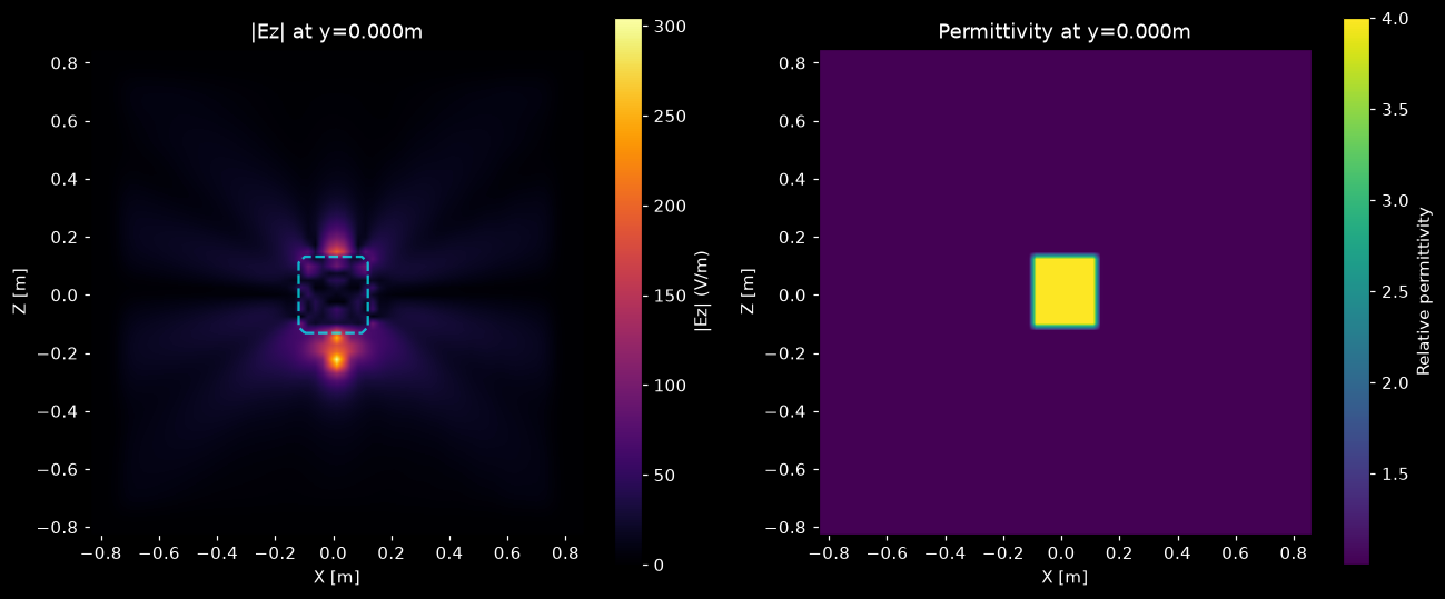Ez magnitude and permittivity on the y = 0 plane for a dipole below a dielectric box

What each step does #

Describe the scene
A Scene holds the physical domain, the grid, the boundary and every object in it. Domain.bounds is the physical region in metres; the 8 PML layers are added outside it, so the computed grid is 52 + 16 = 68 cells per axis. Structure pairs a geometry (Box) with a Material. The box position is a PyTorch tensor, so the scene is differentiable with respect to it. See Scene, Simulation, Result.
Add a source and monitors
PointDipole injects a current at one point with a GaussianPulse time signal centred at 1.5 GHz. FluxMonitor integrates the Poynting vector over a plane; normal_direction="-" counts power that flows toward negative z. PointMonitor records the field phasor at one point. See Sources and monitors.
Run the simulation
Simulation.fdtd picks the time step and the number of steps for you: here 5387 steps of 11.1 ps, limited by 30 steps per period of the highest frequency the pulse contains. The solver accumulates a discrete Fourier transform at each requested frequency while it steps. full_field_dft=True also keeps the spectrum of the whole grid, which result.plot.field needs.
Read the result
result.monitor(name) returns a dictionary. Flux monitors carry "flux"; point monitors carry "data" (the complex phasor) and one key per field component. All values are PyTorch tensors on the GPU. See Read and plot results.
Take a gradient
loss.backward() runs Maxwell's native CUDA adjoint solve and fills box_z.grad. Any scalar built from monitor outputs can be the loss. See Differentiability.

Tip

If you do not need gradients, build the scene with plain floats (position=(0.0, 0.0, 0.0)) or run under torch.no_grad(). The forward run alone takes a few seconds.