Dipole near a dielectric box
Measure the total power a dipole radiates next to a dielectric box with a closed set of flux faces, and refine the grid until the answer converges.
This tutorial takes the quickstart scene further. It encloses the dipole and the box with six flux faces to measure the total radiated power and where it goes, compares it with the dipole alone, and repeats the run on finer grids. The result shows why the quickstart's 2.5 cm grid is fine for a first run but not for numbers you report. The scene follows benchmark/scenes/dipole/dipole_dielectric_box.py in the Maxwell repository.
You need a CUDA GPU. The script runs eight simulations in about 50 seconds on a recent GPU.
The setup#
- A z-polarized
PointDipoleat z = -0.20 m radiates a 1.5 GHz pulse (free-space wavelength 0.2 m). A 0.24 m cube witheps_r = 4sits above it, centred at the origin. Inside the cube the wavelength is 0.1 m. - Six
FinitePlaneMonitorfaces form a 0.8 m cube around both. Each face records its two tangential E and H components and integrates the Poynting vector (compute_flux=True), withnormal_directionpointing out of the cube. The six fluxes add up to the total radiated power. - Each grid runs twice, with and without the dielectric box. The ratio of the two totals tells you how the box changes the power the dipole radiates. Taking a ratio removes the source normalization.
Full script#
import time
import matplotlib.pyplot as plt
import witwin.maxwell as mw

f0 = 1.5e9                 # Hz, free-space wavelength 0.2 m
half = 0.64                # half-width of the domain, m
box_half = 0.40            # half-width of the power box, m

def build_scene(dl, with_box=True):
    scene = mw.Scene(
        domain=mw.Domain(bounds=((-half, half),) * 3),
        grid=mw.GridSpec.uniform(dl),
        boundary=mw.BoundarySpec.pml(num_layers=8),
        subpixel_samples=mw.SubpixelSpec(samples=3, averaging="polarized"),
        device="cuda",
    )
    if with_box:
        scene.add_structure(
            mw.Structure(
                name="dielectric_box",
                geometry=mw.Box(position=(0.0, 0.0, 0.0), size=(0.24, 0.24, 0.24)),
                material=mw.Material(eps_r=4.0),
            )
        )
    scene.add_source(
        mw.PointDipole(
            name="dipole",
            position=(0.0, 0.0, -0.20),
            polarization="Ez",
            source_time=mw.GaussianPulse(frequency=f0, fwidth=0.5e9),
        )
    )
    # Six finite faces that enclose the dipole and the box. Each one integrates the
    # Poynting vector over its own rectangle, pointing out of the enclosed volume.
    for axis, (tangential_a, tangential_b) in (("x", ("Ey", "Ez")), ("y", ("Ex", "Ez")), ("z", ("Ex", "Ey"))):
        h_fields = tuple("H" + c[1] for c in (tangential_a, tangential_b))
        for sign in ("+", "-"):
            center = [0.0, 0.0, 0.0]
            center["xyz".index(axis)] = box_half if sign == "+" else -box_half
            size = [2 * box_half] * 3
            size["xyz".index(axis)] = 0.0
            scene.add_monitor(
                mw.FinitePlaneMonitor(
                    f"face_{sign}{axis}",
                    position=tuple(center),
                    size=tuple(size),
                    fields=(tangential_a, tangential_b) + h_fields,
                    frequencies=(f0,),
                    compute_flux=True,
                    normal_direction=sign,
                )
            )
    scene.add_monitor(mw.PlaneMonitor("field_xz", axis="y", position=0.0, fields=("Ez",), frequencies=(f0,)))
    return scene

FACES = [f"face_{sign}{axis}" for axis in "xyz" for sign in "+-"]

def run(dl, with_box=True):
    result = mw.Simulation.fdtd(build_scene(dl, with_box), frequencies=[f0]).run()
    powers = {name: float(result.monitor(name)["flux"]) for name in FACES}
    return result, powers

print("   dl (m)   P_box / P_free   up     down   sides")
for dl in (0.025, 0.02, 0.0125, 0.01):
    _, free = run(dl, with_box=False)
    result, p = run(dl)
    total = sum(p.values())
    sides = total - p["face_+z"] - p["face_-z"]
    print(f"  {dl:6.4f}       {total / sum(free.values()):.3f}       "
          f"{p['face_+z'] / total:5.1%}  {p['face_-z'] / total:5.1%}  {sides / total:5.1%}")

# Plot |Ez| from the finest run (the last `result`), cropped to the physical domain.
plane = result.monitor("field_xz")
ez = plane["Ez"].abs().cpu().numpy()
fig, ax = plt.subplots(figsize=(5, 4.2), layout="constrained")
mesh = ax.pcolormesh(plane["x"], plane["z"], ez.T, cmap="magma", vmax=0.2 * ez.max(), shading="auto")
ax.add_patch(plt.Rectangle((-0.12, -0.12), 0.24, 0.24, fill=False, color="white", linestyle="--"))
ax.add_patch(plt.Rectangle((-box_half, -box_half), 2 * box_half, 2 * box_half, fill=False, color="cyan", linewidth=0.8))
ax.plot([0.0], [-0.20], "w^")
ax.set_xlim(-half, half)
ax.set_ylim(-half, half)
ax.set_aspect("equal")
ax.set_xlabel("x (m)")
ax.set_ylabel("z (m)")
fig.colorbar(mesh, ax=ax, label="|Ez| at 1.5 GHz (clipped)")
fig.savefig("dipole_box_convergence.png", dpi=110)
Expected output#
dl (m) P_box / P_free up down sides
0.0250 0.981 12.4% 23.1% 64.5%
0.0200 0.922 12.2% 21.9% 65.9%
0.0125 0.821 13.4% 17.2% 69.5%
0.0100 0.817 13.7% 17.5% 68.9%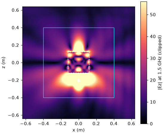 |Ez| in the y = 0 plane at 1 cm resolution. The dipole is below the dashed dielectric cube; the solid square is the flux box
Reading the result#
- The box lowers the radiated power. On the finest grids, the dipole radiates about 18% less with the box present (
P_box / P_free= 0.82). The box scatters part of the field back onto the dipole, which changes the power the dipole delivers. - Most power leaves sideways. A z-polarized dipole radiates mostly in the horizontal plane, so about 69% leaves through the four side faces. The
upanddowncolumns are the fractions through the top and bottom faces. - The coarse grids are wrong by up to 20%. At 2.5 cm, the cube has only four cells per wavelength inside the dielectric, and the ratio comes out as 0.98 instead of 0.82. Between 1.25 cm and 1 cm, the ratio changes by 0.5% and the splits by less than half a percentage point, so 1.25 cm (eight cells per wavelength inside the dielectric) is converged for this scene.
A practical rule: use at least 10 cells per wavelength in the densest material for a first look, then halve the cell size once and check that the numbers you care about stop changing. See Grid, units and boundaries.
Notes on the monitors#
FinitePlaneMonitorfaces record E and H together and compute flux when they hold the four tangential components, as here.- The flux values are spectral powers of the pulse at 1.5 GHz, so compare them as ratios, as done here. For absolute power per unit source amplitude, run with
spectral_sampler=mw.SpectralSampler(normalize_source=True). ClosedSurfaceMonitor.box(...)builds the same six faces in one call for far-field projection; see Far field, directivity and RCS.
Next steps#
- Inverse design of a dielectric lens turns the box into a design region.
- Set up grids and boundaries covers non-uniform and automatic grids, which refine only where the material needs it.