Rectangular waveguide S-parameters

Build a PEC rectangular waveguide, terminate it with two wave ports, sweep them, and check the S-matrix against the analytic TE10 mode.

This tutorial measures the S-parameters of a straight, air-filled rectangular waveguide between two WavePorts. A straight guide has a known answer: no reflection, full transmission, and a transmission phase set by the TE10 propagation constant. That makes it the right first check before you model a real waveguide device. The scene is adapted from benchmark/scenes/rf/rectangular_waveguide.py in the Maxwell repository.

You need a CUDA GPU. The script runs in about 40 seconds on a recent GPU.

The setup #

The guide is 0.6 m wide (y) and 0.3 m high (z), so the TE10 cutoff is fc = c / (2a), about 250 MHz.
Four PEC boxes form the walls. They run through the PML at both ends, so the guide looks infinitely long and the open wall ends do not reflect.
Two wave ports sit 0.6 m apart at x = -0.3 m and x = +0.3 m. Each port's reference plane is at its own position.
A port sweep drives each port in turn at six frequencies from 1.2 fc to 2.2 fc, where only TE10 propagates.

Full script #

import numpy as np
import matplotlib.pyplot as plt
import witwin.maxwell as mw
from witwin.maxwell.constants import C_0
 
a, b = 0.60, 0.30          # inner width (y) and height (z) of the guide, m
dl = 0.025                 # cell size, m
pml = 8                    # PML layers on each face
fc = C_0 / (2 * a)         # TE10 cutoff frequency, Hz (about 250 MHz)
 
scene = mw.Scene(
    domain=mw.Domain(bounds=((-0.6, 0.6), (-0.5, 0.5), (-0.35, 0.35))),
    grid=mw.GridSpec.uniform(dl),
    boundary=mw.BoundarySpec.pml(num_layers=pml),
    device="cuda",
)
 
# Four PEC walls. They run through the PML on both ends so the guide looks infinitely long.
wall_length = 2 * (0.6 + pml * dl) + 8 * dl
for name, position, size in (
    ("wall_y_high", (0.0, 0.40, 0.0), (wall_length, 0.20, 0.70)),
    ("wall_y_low", (0.0, -0.40, 0.0), (wall_length, 0.20, 0.70)),
    ("wall_z_high", (0.0, 0.0, 0.25), (wall_length, 0.60, 0.20)),
    ("wall_z_low", (0.0, 0.0, -0.25), (wall_length, 0.60, 0.20)),
):
    scene.add_structure(
        mw.Structure(name=name, geometry=mw.Box(position=position, size=size), material=mw.Material.pec())
    )
 
# One wave port at each end, 0.6 m apart, both looking into the guide.
for name, x, direction in (("left", -0.3, "+"), ("right", 0.3, "-")):
    scene.add_port(
        mw.WavePort(
            name,
            position=(x, 0.0, 0.0),
            size=(0.0, a, b),
            direction=direction,
            reference_plane=x,
            modes=(mw.WaveModeSpec("te", polarization="Ez"),),
        )
    )
 
freqs = tuple(float(f) for f in np.linspace(1.2 * fc, 2.2 * fc, 6))
result = mw.Simulation.fdtd(
    scene,
    frequencies=freqs,
    excitations=mw.PortSweep(),
    run_time=mw.TimeConfig.auto(steady_cycles=8, transient_cycles=16),
).run()
 
net = result.network
S = net.s.detach().cpu().numpy()          # shape (6, 2, 2)
print("channels:", net.port_names)
 
length = 0.6
beta = np.sqrt((2 * np.pi * np.array(freqs) / C_0) ** 2 - (np.pi / a) ** 2)
expected_phase = np.angle(np.exp(1j * beta * length))
for i, f in enumerate(freqs):
    print(
        f"{f / 1e6:6.1f} MHz  |S11| = {abs(S[i, 0, 0]):.3f}  |S21| = {abs(S[i, 1, 0]):.3f}  "
        f"arg S21 = {np.angle(S[i, 1, 0]):+.3f}  beta*L = {expected_phase[i]:+.3f}"
    )
 
net.save("waveguide_network.pt")
 
f_mhz = np.array(freqs) / 1e6
fig, ax = plt.subplots(figsize=(6, 3.5))
ax.plot(f_mhz, 20 * np.log10(np.abs(S[:, 1, 0])), "o-", label="|S21|")
ax.plot(f_mhz, 20 * np.log10(np.abs(S[:, 0, 0])), "s-", label="|S11|")
ax.set_xlabel("Frequency (MHz)")
ax.set_ylabel("dB")
ax.legend()
ax.grid(True, alpha=0.3)
fig.savefig("waveguide_s_params.png", dpi=110, bbox_inches="tight")

Expected output #

channels: ('left::TE0', 'right::TE0')
 299.8 MHz  |S11| = 0.014  |S21| = 0.987  arg S21 = +2.082  beta*L = +2.084
 349.8 MHz  |S11| = 0.001  |S21| = 1.000  arg S21 = +3.081  beta*L = +3.078
 399.7 MHz  |S11| = 0.003  |S21| = 1.000  arg S21 = -2.356  beta*L = -2.359
 449.7 MHz  |S11| = 0.005  |S21| = 1.000  arg S21 = -1.577  beta*L = -1.581
 499.7 MHz  |S11| = 0.005  |S21| = 1.000  arg S21 = -0.834  beta*L = -0.842
 549.6 MHz  |S11| = 0.001  |S21| = 1.000  arg S21 = -0.116  beta*L = -0.127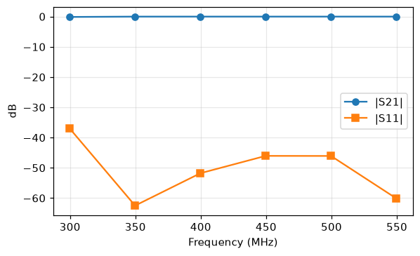

|S21| close to 0 dB and |S11| below -35 dB from 300 to 550 MHz

Reading the result #

Transmission. |S21| is 1.000 to three digits above 1.4 fc. Close to cutoff (300 MHz), the mode is slow and the grid resolves it less well, so |S21| drops to 0.987.
Reflection. |S11| stays below 0.015 (below -35 dB), which is the numerical reflection of the ports and the PML.
Phase. arg S21 matches beta * L to within 0.011 rad, where beta = sqrt(k0² - (pi / a)²) is the TE10 propagation constant. The sign is positive because Maxwell uses the exp(-i omega t) phasor convention; tools that use exp(+j omega t) report the conjugate.
Channels. Each port mode is a network channel named "<port>::<mode>", here left::TE0 and right::TE0.

Exporting the network #

net.save(path) writes a snapshot that mw.NetworkData.load(path) reads back. To write a Touchstone file, first renormalize: a WavePort's reference impedance is the TE10 wave impedance, which changes with frequency, and a Touchstone file holds one value per port. net.to_touchstone(...) raises ValueError otherwise.

net.renormalize(50.0).to_touchstone("waveguide.s2p")

The renormalized S-matrix describes the guide as seen from 50 Ω ports, so it shows large reflections. That is correct for that reference, not a simulation error.

Next steps #

Put a device between the ports (an iris, a post or a dielectric block) and compare its S-parameters with the straight guide.
Read Mode ports and S-parameters for port placement rules and the NetworkData methods.

The setup#

Full script#

Expected output#

Reading the result#

Exporting the network#

Next steps#