Plane-wave scattering from a dielectric sphere
Illuminate a dielectric sphere with a plane wave, measure reflected and transmitted power with flux monitors, and plot the field in a cut plane.
This tutorial sends a plane wave onto a dielectric sphere and measures where the power goes. You run the scene twice, once in vacuum and once with the sphere, and compare the power that crosses two planes. The comparison is the usual way to measure reflection and transmission in FDTD, because the vacuum run tells you exactly what the source delivered. The scene is adapted from benchmark/scenes/planewave/planewave_dielectric_sphere.py in the Maxwell repository.
You need a CUDA GPU. Both runs together take about 10 seconds on a recent GPU.
The setup#
- A sphere of radius 0.12 m with
eps_r = 4sits at the origin. At 1 GHz the free-space wavelength is 0.3 m, so the sphere is about one wavelength across inside the dielectric. - A
PlaneWavetravels toward +z with E along x. Without aninjectionargument, it is injected on a plane near the -z boundary. flux_forwardat z = +0.3 m measures power that passes the sphere.flux_backwardat z = -0.3 m points toward -z (normal_direction="-"), so it counts power travelling back toward the source.- A
PlaneMonitorrecords Ex in the y = 0 plane for the plot.SubpixelSpecaverages the permittivity in cells cut by the sphere surface, so the curved surface is not a hard staircase.
Full script#
import matplotlib.pyplot as plt
import witwin.maxwell as mw

f0 = 1.0e9                 # Hz, free-space wavelength 0.3 m
dl = 0.02                  # m, 15 cells per free-space wavelength
half = 0.64                # half-width of the domain, m

def build_scene(with_sphere):
    scene = mw.Scene(
        domain=mw.Domain(bounds=((-half, half),) * 3),
        grid=mw.GridSpec.uniform(dl),
        boundary=mw.BoundarySpec.pml(num_layers=8),
        subpixel_samples=mw.SubpixelSpec(samples=3, averaging="polarized"),
        device="cuda",
    )
    if with_sphere:
        scene.add_structure(
            mw.Structure(
                name="dielectric_sphere",
                geometry=mw.Sphere(position=(0.0, 0.0, 0.0), radius=0.12),
                material=mw.Material(eps_r=4.0),
            )
        )
    scene.add_source(
        mw.PlaneWave(
            direction=(0.0, 0.0, 1.0),        # travels toward +z
            polarization=(1.0, 0.0, 0.0),     # E along x
            source_time=mw.GaussianPulse(frequency=f0, fwidth=0.3e9),
            name="plane_wave",
        )
    )
    scene.add_monitor(mw.PlaneMonitor("field_xz", axis="y", position=0.0, fields=("Ex",), frequencies=(f0,)))
    scene.add_monitor(mw.FluxMonitor("flux_forward", axis="z", position=0.30, frequencies=(f0,)))
    scene.add_monitor(
        mw.FluxMonitor("flux_backward", axis="z", position=-0.30, frequencies=(f0,), normal_direction="-")
    )
    return scene

results = {}
for with_sphere in (False, True):
    results[with_sphere] = mw.Simulation.fdtd(build_scene(with_sphere), frequencies=[f0]).run()

def flux(result, name):
    return float(result.monitor(name)["flux"])

incident = flux(results[False], "flux_forward")
# The backward plane also sees the incident wave pass through it, so subtract the vacuum run.
reflected = flux(results[True], "flux_backward") - flux(results[False], "flux_backward")
transmitted = flux(results[True], "flux_forward")
print(f"incident power:     {incident:.4e}")
print(f"reflected power:    {reflected:.4e}  ({reflected / incident:.2%} of incident)")
print(f"transmitted power:  {transmitted:.4e}  ({transmitted / incident:.2%} of incident)")
print("time steps:", results[True].stats()["steps_run"])

planes = {key: res.monitor("field_xz") for key, res in results.items()}
vmax = float(planes[True]["Ex"].abs().max())
fig, axes = plt.subplots(1, 2, figsize=(9, 4), sharey=True, layout="constrained")
for ax, with_sphere in zip(axes, (False, True)):
    plane = planes[with_sphere]
    ex = plane["Ex"].abs().cpu().numpy()              # |Ex| phasor magnitude, shape (Nx, Nz)
    mesh = ax.pcolormesh(plane["x"], plane["z"], ex.T, cmap="magma", vmin=0.0, vmax=vmax, shading="auto")
    if with_sphere:
        ax.add_patch(plt.Circle((0.0, 0.0), 0.12, fill=False, color="white", linestyle="--"))
    ax.set_xlim(-half, half)
    ax.set_ylim(-half, half)
    ax.set_aspect("equal")
    ax.set_title("with sphere" if with_sphere else "vacuum")
    ax.set_xlabel("x (m)")
axes[0].set_ylabel("z (m)")
fig.colorbar(mesh, ax=axes, shrink=0.8, label="|Ex| at 1 GHz")
fig.savefig("planewave_sphere_ex.png", dpi=110)
Expected output#
incident power: 2.3465e-04
reflected power: 3.6426e-06 (1.55% of incident)
transmitted power: 2.2702e-04 (96.75% of incident)
time steps: 3937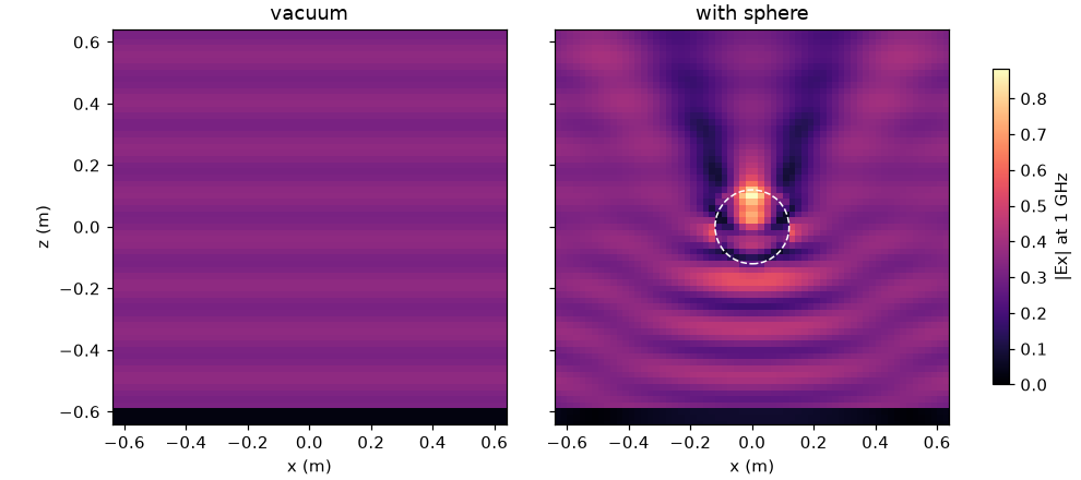 |Ex| in the y = 0 plane: uniform in vacuum, focused behind the sphere and with a standing-wave pattern in front of it
Reading the result#
- Power units. Flux values are spectral powers of the pulse at 1 GHz through each plane, so only their ratios are meaningful here. Use them as fractions of the vacuum run.
- Reflection. About 1.5% of the incident power comes back through the plane at z = -0.3 m. The flux monitor spans the whole plane, so this counts every backward-scattered direction that crosses it.
- Transmission. About 97% crosses the plane at z = +0.3 m. The sphere is lossless, so the missing 1.7% is scattered at angles that miss both planes and is absorbed by the PML at the sides.
- Field map. The sphere acts as a lens and focuses the field just behind it. In front of it, the reflected wave interferes with the incident wave and forms the standing-wave ripples. The dark strip at the bottom lies behind the injection plane, where the source sends no field.
The vacuum map also shows a weak ripple along z from small numerical reflections at the domain edges. Subtracting the vacuum run removes their contribution, and the incident wave itself, from flux_backward.
Variations#
- Change
eps_ror the radius and watch the reflection and the focus move. - To separate the scattered field from the incident field, use a TFSF box (
injection=mw.TFSF(bounds=...)); see Choose sources and waveforms. - To get a scattering pattern, record a
ClosedSurfaceMonitorand project it; see Far field, directivity and RCS.