Inverse design of a dielectric lens

Optimize the permittivity inside a design box with gradients from the native adjoint, so a dipole's field is focused onto a target point.

This tutorial uses gradients to design a dielectric block. A dipole radiates toward a target point on the other side of a design box. The permittivity inside the box is free to vary between air and eps_r = 4, and an optimizer changes it to make the field at the target as strong as possible. After ten steps the optimizer has drawn a round lens on its own.

You need a CUDA GPU. Each step runs one forward simulation and one adjoint simulation; on a recent GPU a step takes about 15 seconds and the whole script about 2.5 minutes. For the background, read Differentiability first.

The setup #

A MaterialRegion named lens fills a 0.24 × 0.24 × 0.08 m box at the origin. Its density tensor has 12 × 12 × 4 samples, interpolated over the box. Density 0 is air and density 1 is eps_r = 4 (eps_bounds=(1.0, 4.0)).
An x-polarized PointDipole at z = -0.15 m radiates toward the box at 1.5 GHz (wavelength 0.2 m).
The objective is |Ex|² at a PointMonitor at z = +0.15 m, the far side of the box.
The optimizer works on unconstrained logits; torch.sigmoid(logits) turns them into a density between 0 and 1. It starts from density 0.5 everywhere.

Full script #

import time
import torch
import matplotlib.pyplot as plt
import witwin.maxwell as mw
 
f0 = 1.5e9                 # Hz, free-space wavelength 0.2 m
dl = 0.02                  # m, 10 cells per free-space wavelength
design_shape = (12, 12, 4) # density samples over the design box (x, y, z)
 
def build_scene(density):
    scene = mw.Scene(
        domain=mw.Domain(bounds=((-0.3, 0.3), (-0.3, 0.3), (-0.3, 0.3))),
        grid=mw.GridSpec.uniform(dl),
        boundary=mw.BoundarySpec.pml(num_layers=8),
        device="cuda",
    )
    scene.add_material_region(
        mw.MaterialRegion(
            name="lens",
            geometry=mw.Box(position=(0.0, 0.0, 0.0), size=(0.24, 0.24, 0.08)),
            density=density,
            eps_bounds=(1.0, 4.0),          # density 0 -> air, density 1 -> eps_r = 4
        )
    )
    scene.add_source(
        mw.PointDipole(
            name="feed",
            position=(0.0, 0.0, -0.15),
            polarization="Ex",
            source_time=mw.GaussianPulse(frequency=f0, fwidth=0.4e9),
        )
    )
    scene.add_monitor(mw.PointMonitor("target", (0.0, 0.0, 0.15), fields=("Ex",)))
    return scene
 
def intensity_at_target(density):
    result = mw.Simulation.fdtd(build_scene(density), frequencies=[f0]).run()
    return result.monitor("target")["data"].abs().square()
 
# Optimize an unconstrained tensor; the sigmoid keeps the density between 0 and 1.
logits = torch.zeros(design_shape, device="cuda", requires_grad=True)
optimizer = torch.optim.Adam([logits], lr=0.5)
 
with torch.no_grad():
    baseline = float(intensity_at_target(torch.zeros(design_shape, device="cuda")))
print(f"empty design region: |Ex|^2 = {baseline:.4g}")
 
history = []
for step in range(10):
    t0 = time.perf_counter()
    optimizer.zero_grad()
    intensity = intensity_at_target(torch.sigmoid(logits))
    (-intensity).backward()                 # maximize the intensity at the target
    optimizer.step()
    history.append(float(intensity.detach()) / baseline)
    print(f"step {step}: |Ex|^2 / empty = {history[-1]:.3f}   ({time.perf_counter() - t0:.1f} s)")
 
density = torch.sigmoid(logits).detach().cpu()
print("final mean density:", round(float(density.mean()), 3))
 
fig, axes = plt.subplots(1, 2, figsize=(8, 3.5), layout="constrained")
axes[0].plot(range(len(history)), history, "o-")
axes[0].set_xlabel("Iteration")
axes[0].set_ylabel("|Ex|² at target / empty region")
axes[0].grid(True, alpha=0.3)
image = axes[1].imshow(density[:, :, design_shape[2] // 2].T, origin="lower", cmap="gray_r",
                       vmin=0.0, vmax=1.0, extent=(-0.12, 0.12, -0.12, 0.12))
axes[1].set_title("Density, middle z slice")
axes[1].set_xlabel("x (m)")
axes[1].set_ylabel("y (m)")
fig.colorbar(image, ax=axes[1])
fig.savefig("inverse_design.png", dpi=110)

Expected output #

empty design region: |Ex|^2 = 4649
step 0: |Ex|^2 / empty = 1.775   (15.5 s)
step 1: |Ex|^2 / empty = 3.563   (13.5 s)
step 2: |Ex|^2 / empty = 4.834   (13.8 s)
step 3: |Ex|^2 / empty = 5.562   (14.8 s)
step 4: |Ex|^2 / empty = 5.989   (14.1 s)
step 5: |Ex|^2 / empty = 6.272   (14.3 s)
step 6: |Ex|^2 / empty = 6.475   (16.4 s)
step 7: |Ex|^2 / empty = 6.622   (14.5 s)
step 8: |Ex|^2 / empty = 6.724   (13.6 s)
step 9: |Ex|^2 / empty = 6.798   (13.8 s)
final mean density: 0.431

Timings depend on your GPU. The intensity values can differ slightly between GPUs and driver versions.

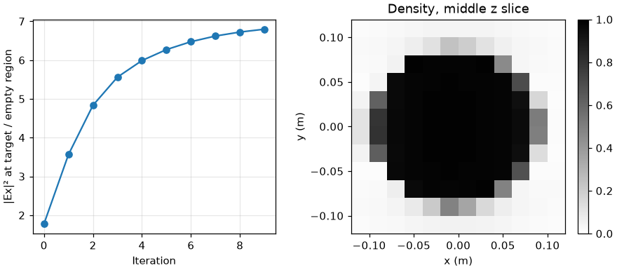Left: intensity at the target rising from 1.8 to 6.8 times the empty-region value over ten steps. Right: the optimized density, a solid disk about 0.15 m across surrounded by air

How it works #

The scene is rebuilt every step. build_scene(density) puts the current density tensor into a new MaterialRegion. Because the tensor depends on logits, the result carries an autograd graph back to logits.
The backward pass is a second simulation. (-intensity).backward() runs Maxwell's native CUDA adjoint: it replays the time stepping backward from stored checkpoints and returns the gradient of the intensity with respect to every density sample in one pass, no matter how many samples there are.
Any PyTorch optimizer works. The loss is the negative intensity because Adam minimizes.
The baseline uses torch.no_grad(). The reference run needs no gradient, so it records no autograd graph.

Reading the result #

The design starts as a uniform eps_r = 2.5 slab, which already gives 1.8 times the empty-region intensity. The optimizer then fills the centre and empties the edges, forming a convex lens that focuses the dipole's beam on the target: 6.8 times the empty-region intensity after ten steps. More steps keep improving it slowly.

Make it manufacturable #

The density here is still grey in places (between 0 and 1). For a design you can build:

Add projection_beta= to the MaterialRegion and raise it over the iterations (for example 2, 4, 8, 16) to push the density toward 0 or 1.
Add filter_radius= (metres) to smooth out features smaller than your fabrication limit.

Next steps #

Differentiability lists every input you can optimize and the limits.
Batch and multi-GPU runs evaluates several densities at once, with gradients.

The setup#

Full script#

Expected output#

How it works#

Reading the result#

Make it manufacturable#

Next steps#